Tracking Image Features
Tracking Image Features
The task of tracking image features is very challenging because we want to identify and track reliable features in an image, also known as keypoints, through a sequence of images.
Corner Detectors
A corner can be located by following these steps:
- Calculate the gradient for a small window of the image, using sobel-x and sobel-y operators (without applying binary thesholding).
- Use vector addition to calculate the magnitude and direction of the total gradient from these two values.
- Apply this calculation as you slide the window across the image, calculating the gradient of each window. When a big variation in the direction & magnitude of the gradient has been detected - a corner has been found!
Intensity Gradient and Filtering
Harris Corner Detector
Overview of Popular Keypoint Detectors
Depending on which type of keypoints we want to detect there are a variety of different keypoint detection algorithms. There are four basic transformation types we need to think about when selecting a suitable keypoint detector:
- Rotation
- Scale change
- Intensity change
- Affine transformation
Applications of keypoint detection include such things as object recognition and tracking, image matching and panoramic stitching as well as robotic mapping and 3D modeling. In addition to invariance under the transformations mentioned above, detectors can be compared for their detection performance and their processing speed.
The Harris detector along with several other "classics" belongs to a group of traditional detectors, which aim at maximizing detection accuracy. In this group, computational complexity is not a primary concern. The following list shows a number of popular classic detectors :
- 1988 Harris Corner Detector (Harris, Stephens)
- 1996 Good Features to Track (Shi, Tomasi)
- 1999 Scale Invariant Feature Transform (Lowe)
- 2006 Speeded Up Robust Features (Bay, Tuytelaars, Van Gool)
In recent years, a number of faster detectors have been developed which aim at real-time applications on smartphones and other portable devices. The following list shows the most popular detectors belonging to this group:
- 2006 Features from Accelerated Segment Test (FAST) (Rosten, Drummond)
- 2010 Binary Robust Independent Elementary Features (BRIEF) (Calonder, et al.)
- 2011 Oriented FAST and Rotated BRIEF (ORB) (Rublee et al.)
- 2011 Binary Robust Invariant Scalable Keypoints (BRISK) (Leutenegger, Chli, Siegwart)
- 2012 Fast Retina Keypoint (FREAK) (Alahi, Ortiz, Vandergheynst)
- 2012 KAZE (Alcantarilla, Bartoli, Davidson)
Features from Accelerated Segments Test (FAST)
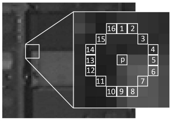
Finds keypoints by comparing the brightness levels in a given pixel area. Given a pixel \(p\) in an image, FAST compares the brigthness of \(p\) to a set of 16 surrounding pixels that are in a small circle around \(p\).
Each pixel in this circle is then sorted into three classes, depending on the brightness of the pixel \(I_p\) (intensity of pixel \(p\)):
- brighter than \(p\):
- darker than \(p\)
- similar to \(p\)
So if the brithness of a pixel is \(I_p\), then for a given threshold \(h\) brither pixels will be those, whose brithness exceeds \(I_p + h\). Darker pixels will be those whose brithness is below \(I_p - h\), and similar pixels will be those whose brithness lie in-between those values. Once the pixels are classified into the three classes mentiond above, pixel \(p\) is selected as a keypoint if more than eight connected pixels on the circle are either darker or brighter than \(p\).
The reason FAST is so efficient, is that it takes advantage of the fact that the same result can be achieved by comparing \(p\) to only four equidistant pixels in the circle, instead of all 16 surrounding pixels. For example, we only have to compare \(p\) to pixels 1, 5, 9, and 13. In this case, \(p\) is selected as a keypoint if there are at least a pair of consecutive pixels that are either brighter or darker than \(p\). This optimization reduces the time required to search an entire image for keypoints by a factor of four.
These keypoints are providing us with informatrion, about where in the image there is a change in intensity. Such regions usually determine an edge of some kind, which is why the keypoints found by FAST, give us information about the location of object defining edges in an image. However, one thing to note is that these keypoints only give us the location of an edge, and don't include any information about the direction of the change of intensity. So we can not distinguish between horizontal and vertical edges, for example. However, this directionality can be useful in some cases.
Now that we know how ORB uses FAST to locates the key points in an image, we can look at how ORB uses the BRIEF algorithm to convert these keypoints into feature vectors, also known as keypoint descriptors.
Descriptors (Feature Vectors)
Descriptors also known als feature vectors provide distinctive information on the surrounding area of a keypoint. The literature differentiates between gradient-based descriptors and binary descriptors, with the latter being a relatively new addition with the clear advantage of computational speed.
- An example of a gradient-based descriptor is the Scale Invariant Feature Transform (SIFT).
- A representative of binary descriptors is the Binary Robust Invariant Scalable Keypoints (BRISK).
HOG Descriptors (SIFT and SURF, etc.)
Binary Descriptors (BRISK, ORB, etc.)
Oriented FAST and Rotated BRIEF (ORB)
ORB is a combination of FAST and BRIEF. FAST is a feature detection algorithm, while BRIEF is a feature vector creation algorithm.
- Keypoint detection using FAST: ORB starts by detecting special regions in an image called keypoints, which is a small region in an image, that is particularly distinctive. Such keypoints are for example corners, where the pixel values sharply change from light to dark.
Note
TODO image showing ORB features.
-
Description using BRIEF: After locating keypoints in an image, ORB calculates a corresponding feature vector for each keypoint. The ORB algorithm creates feature vectors that contain only ones and zeros, which is why they are called binary feature vectors:
\[ V1 = [01011100100110\dots]\\ V2 = [10010100110100\dots]\\ V3 = [11000100101110\dots]\\ \hdots \]
The sequence of ones and zeros varies, according to what a specific keypoint and its surrounding pixel area looks like. The vector represents the pattern of intensity around a keypoint. So multiple feature vectors can be used to identify a larger area and even a specific object in an image.
ORB is not only incredible fast but it is also impervious to noise illumination, and image transformations such as rotations.
References
Text Books and Papers
- Peter Corke, Robotics, Vision, and Control. (Official website) This book has a particular emphasis on computer vision for robotics, but as the title suggests, it goes beyond robot vision.
- Richard Szeliski, Computer Vision: Algorithms and Applications, Springer. The official website provides drafts of recent updates to the book.
- Richard Hartley and Andrew Zisserman, Multiple View Geometry, Cambridge University Press. (Official website)
- David Forsyth and Jean Ponce, Computer Vision: A Modern Approach, Pearson. (Publisher's website)
- Evaluation of Several Feature Detectors/Extractors on Underwater Images towards vSLAM.
Courses
- Udacity Sensor Fusion Engineer Nanodegree
- Stanford University, CS231A: Computer Vision, From 3D Reconstruction to Recognition (Course website)
- Georgia Tech, CS 6476: Computer Vision (Course website)
- MIT, 6.819/6.869: Advances in Computer Vision (Course website)
Online Resources
- OpenCV Tutorials (website)
- OpenCV Python Tutorials (website)
- Medium SIFT (Scale Invariant Feature Transform)
- Detecting lane lines on the road
- Wikipedia Features from Accelerated Segment Test